Switching between space and time: Spatio-temporal analysis with
cubble
Monash University, Australia
2023 May 02
Hi!
A final year PhD student in the Department of Econometrics and Business Statistics
My research centers on exploring multivariate spatio-temporal data with data wrangling and visualisation tool.
Find me on
- Twitter:
huizezhangsh, - GitHub:
huizezhang-sherry, and https://huizezhangsh.netlify.app/
- Twitter:

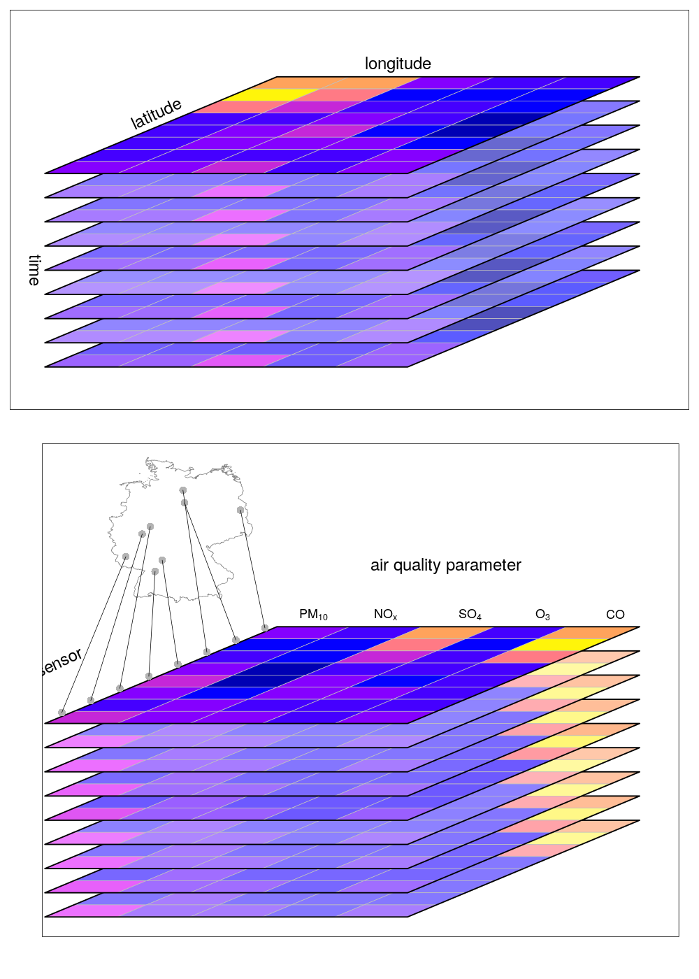
Spatio-temporal data
People can talk about a whole range of different things when they refer to their data as spatio-temporal!
The focus of today will be on vector data.
Example of vector data
Physical sensors that measure the temperature, rainfall, and wind speed & direction

Australian weather station data:
# A tibble: 88 × 6
  id            lat  long  elev name              wmo_id
  <chr>       <dbl> <dbl> <dbl> <chr>              <dbl>
1 ASN00001006 -15.5  128.   3.8 wyndham aero       95214
2 ASN00002032 -17.0  128. 203   warmun             94213
3 ASN00003080 -17.6  124.  77.5 curtin aero        94204
4 ASN00005007 -22.2  114.   5   learmonth airport  94302
5 ASN00006044 -25.9  114.   9   denham             94402
# … with 83 more rows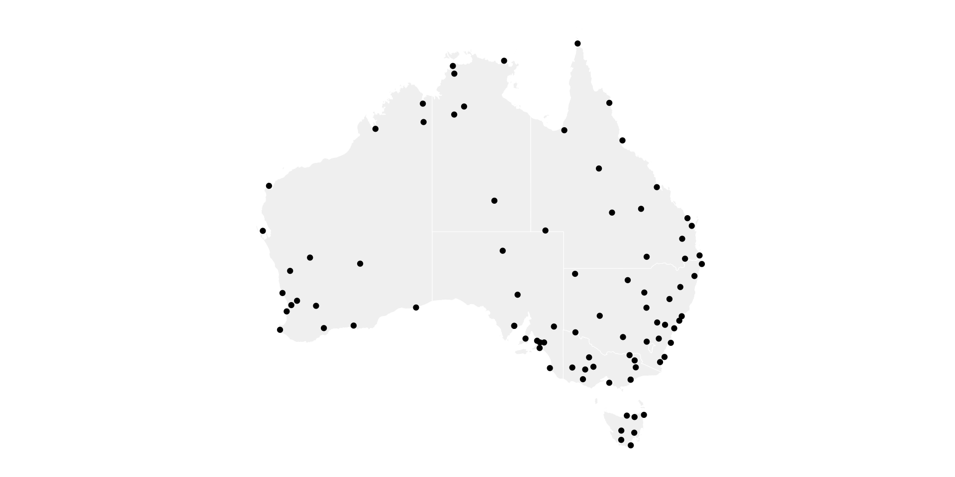
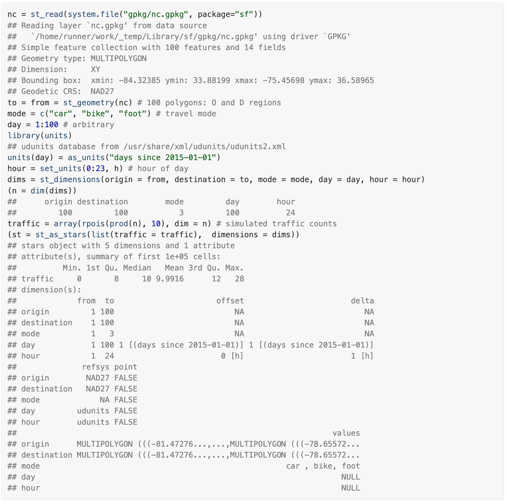
What’s available for spatio-temporal data? - stars
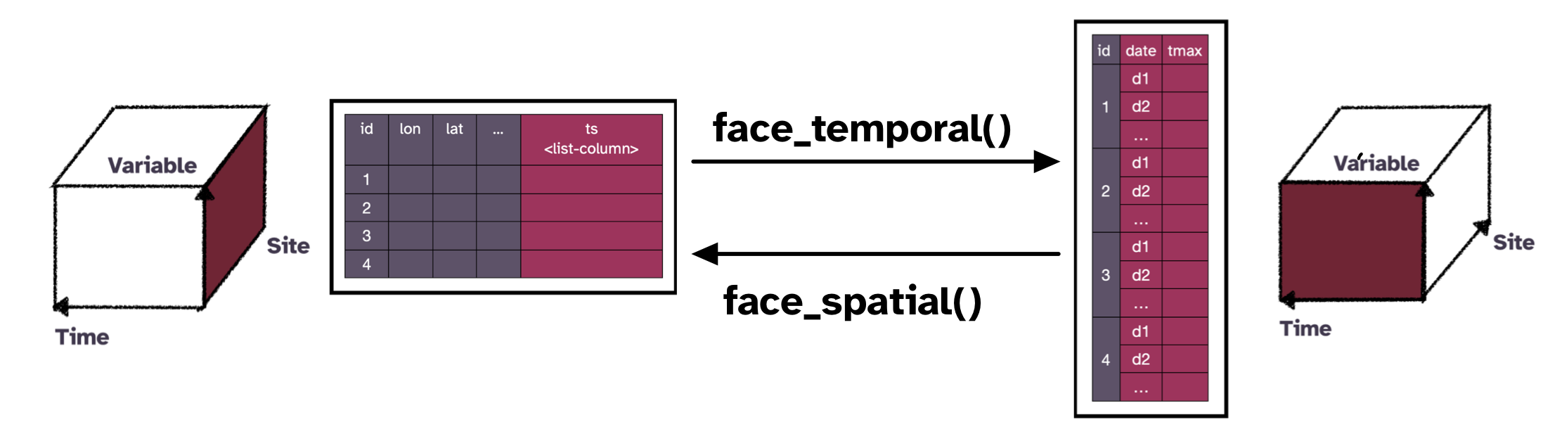
Cubble: a spatio-temporal vector data structure
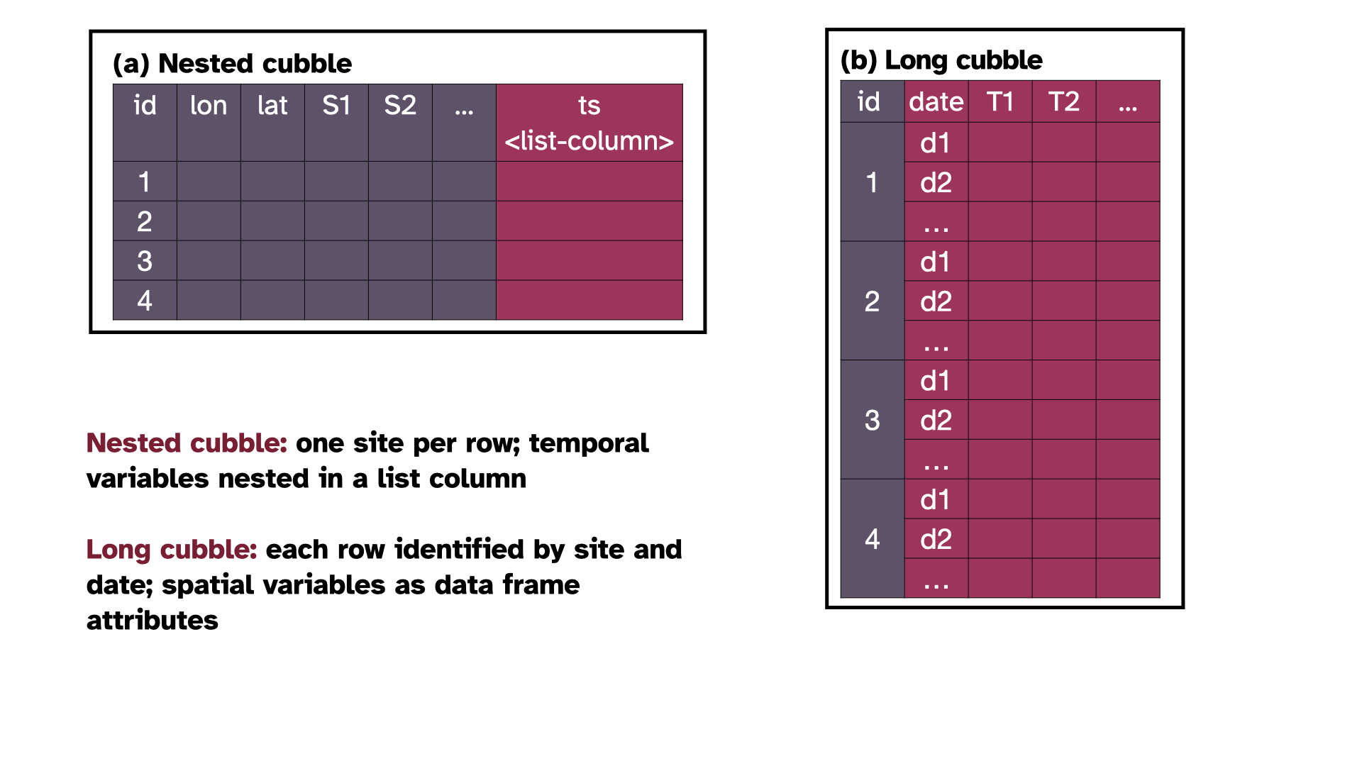
Cubble: a spatio-temporal vector data structure
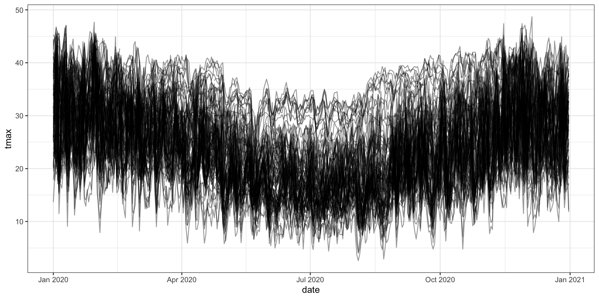
Cubble is a nested object built on tibble that allow easy pivoting between spatial and temporal form.
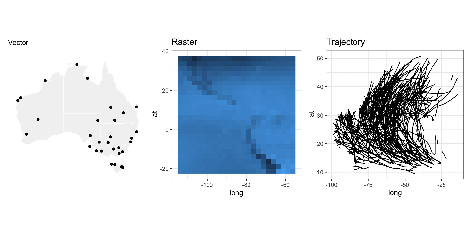
Why do you need a glyph map?
Why do you need a glyph map?
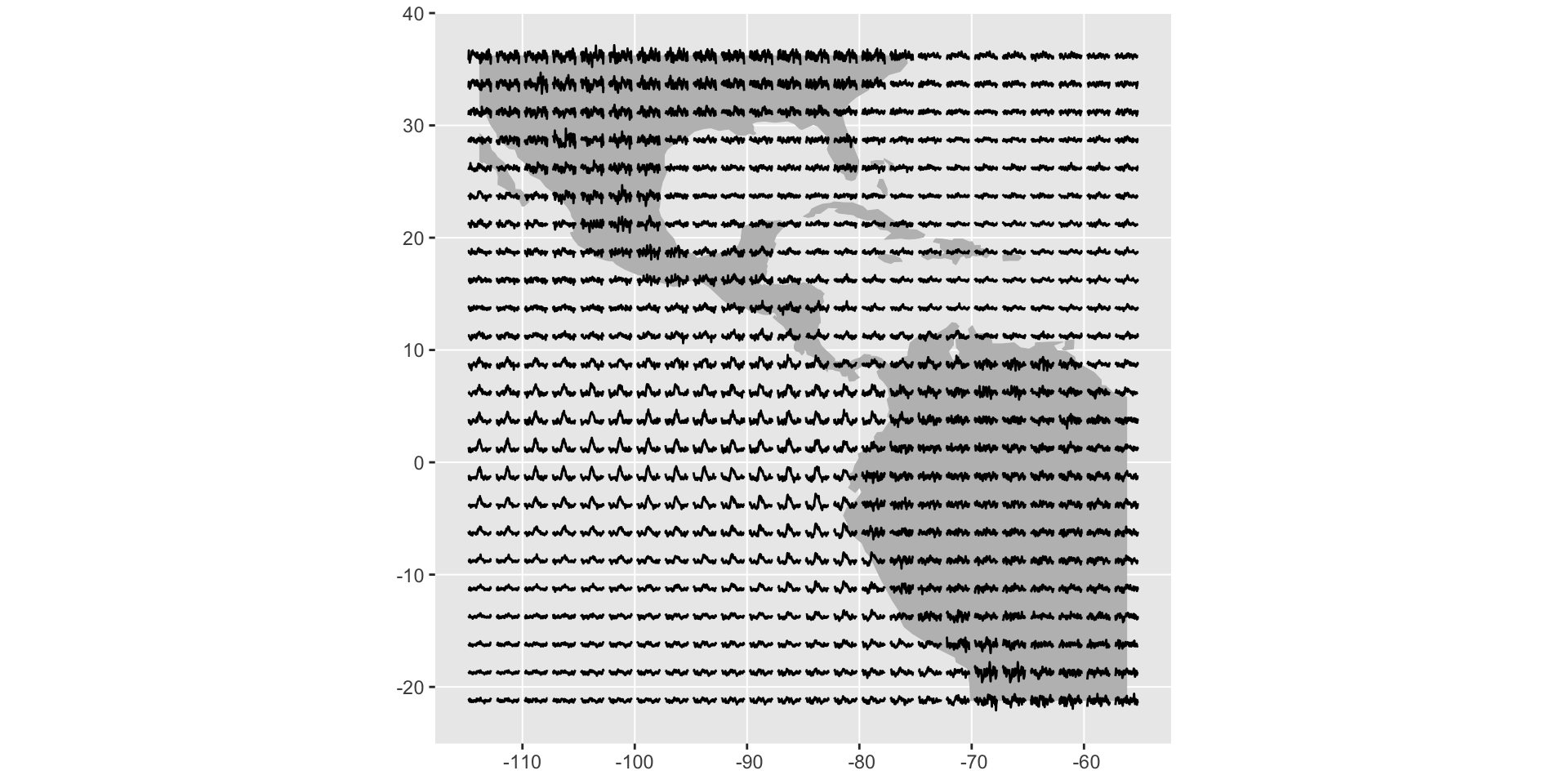
Glyph map transformation
Aggregated temp. by month
cb <- as_cubble(
  list(spatial = stations, temporal = ts),
  key = id, index = date,
  coords = c(long, lat)
)

cb_glyph <- cb %>%
  face_temporal() %>%
  mutate(month = lubridate::month(date)) %>%
  group_by(month) %>%
  summarise(tmax = mean(tmax, na.rm = TRUE)) %>%
  unfold(long, lat)

cb_glyph %>%
  ggplot(aes(x_major = long,
             x_minor = month,
             y_major = lat,
             y_minor = tmax)) +
  geom_sf(data = oz_simp, fill = "grey90",
          color = "white", inherit.aes = FALSE) +
  geom_glyph_box(width = 1.3, height = 0.5) +
  geom_glyph(width = 1.3, height = 0.5) +
  ggthemes::theme_map()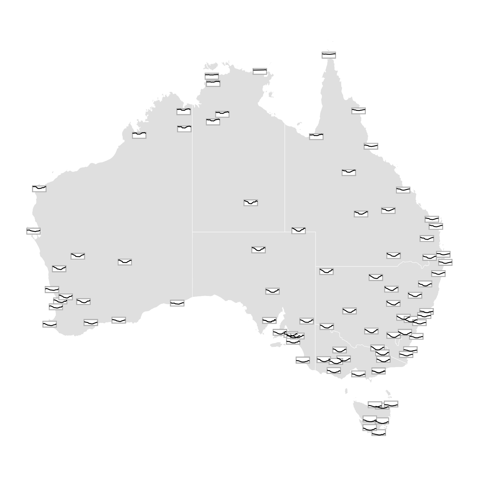
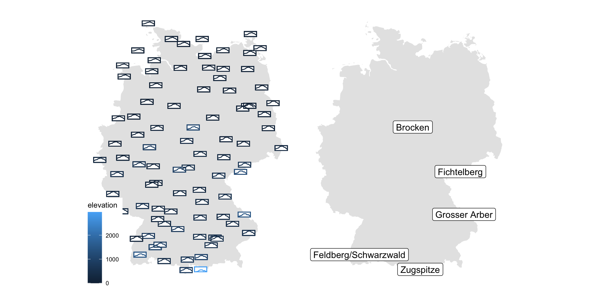
Now with German stations